Program to design L section matching network to match a series RC load

 Program to design L section matching network to match a series RC load

The lumped element model of electronic circuits makes the simplifying assumption that the attributes of the circuit, resistance, capacitance, inductance, and gain, are concentrated into idealized electrical components; resistors, capacitors, and inductors, etc. joined by a network of perfectly conducting wires.

%program to design L section matching network to match a series RC load

clc;

Z1=200-%i*100; // load impedance

R1=200;X1=-100;f=500*100^6;Z0 =100;

B1=(X1+ sqrt (R1/Z0) * sqrt (R1^2+X1^2-(R1*Z0) )) /(R1^2+X1^2);

Two dimensional Fourier transform using Matlab

2-D Fourier transform using 1-D Fourier transform:

The Fourier Transform ( in this case, the 2D Fourier Transform ) is the series expansion of an image function ( over the 2D space domain ) in terms of "cosine" image (orthonormal) basis functions.
The definitons of the transform (to expansion coefficients) and the inverse transform are given below:

 F(u,v) = SUM{ f(x,y)*exp(-j*2*pi*(u*x+v*y)/N) }
    and
 f(x,y) = SUM{ F(u,v)*exp(+j*2*pi*(u*x+v*y)/N) }

    where u = 0,1,2,...,N-1 and v = 0,1,2,...,N-1
   x = 0,1,2,...,N-1 and y = 0,1,2,...,N-1
   j = SQRT( -1 )
   and SUM means double summation  over proper
   x,y or u,v ranges

Program: 

aa=imread('D:\Flower.jpg');          % USE SQAURE IMAGE

aa=rgb2gray(aa)

a1=abs(fft2(aa));                          %Using the inbuilt FFT function for comparison

Program for Discrete Cosine Transform using Matlab

Program for Discrete Cosine Transform using Matlab

The DCT, and in particular the DCT-II, is often used in signal and image processing, especially for lossy compression, because it has a strong "energy compaction" property in typical applications, most of the signal information tends to be concentrated in a few low-frequency components of the DCT.

The discrete cosine transform (DCT) represents an image as a sum of sinusoids of varying magnitudes and frequencies. The dct2 function computes the two-dimensional discrete cosine transform (DCT) of an image. The DCT has the property that, for a typical image, most of the visually significant information about the image is concentrated in just a few coefficients of the DCT. For this reason, the DCT is often used in image compression applications. For example, the DCT is at the heart of the international standard lossy image compression algorithm known as JPEG.

Program:

clc;

x=imread('D:\Flower.jpg');                     %Image Path

a=rgb2gray(x);

figure(1);

imshow(a);

[M N]=size(a);

const=sqrt(2/N);

Program for Histogram Equalization using Matlab

Histogram Equalization

Histogram equalization is a technique for adjusting image intensities to enhance contrast. Let f be a given image represented as a m x n matrix of integer pixel intensities ranging from 0 to L − 1. L is the number of possible intensity values, often 256.

Program: 

clc;

clear all;

close all;

a=imread('D:\sample.jpg');

c=rgb2gray(a);

b=histeq(c);

Program for Bit plane slicing of Image using Matlab

 Program  for  bit plane slicing of Image using Matlab

 Bit extraction or Bit Plane Slicing can be defined as separating a digital image into its bit planes is useful for analyzing the relative importance played by each bit of the image, implying, it determines the adequacy of numbers of bits used to quantize each pixel , useful for image compression. 

For example, for 8-bit data representation there are 8 bit planes: the first bit plane contains the set of the most significant bit, and the 8th contains the least significant bit.

Program:

clc;

a=imread('D:\bird.jpg');

c=rgb2gray(a);

a=double(c);

r=input('which bit of image do you want to see MSB=1 LSB=8 :');

[row col]=size(a);

for x=1:1:row

    for y=1:1:col

        c=dec2bin(a(x,y),8);

        d=c(r);

        w(x,y)=double(d);

        if w(x,y)==49

            w(x,y)==255;

        else

            w(x,y)=0;

        end

    end

end

figure(1)

imshow(uint8(a))

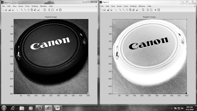
Program for Negative of Image Using Matlab

 Program for Negative of Image Using Matlab

A negative image is a total inversion, in which light areas appear dark and vice versa.
In negative transformation, each value of the input image is subtracted from the L-1 and mapped onto the output image.In this case the following transition has been done.
s = (L – 1) – r
Assuming the input image be 8 bit image , so the number of levels in this image are 256. Putting 256 in the equation, we get this,
s = 255 – r
So each value is subtracted by 255 and the result image has been shown above. So what happens is that , the lighter pixels become dark and the darker picture becomes light. And it results in image negative.

Program for Negative of Image 

clc;

clear all;

a=imread('D:\sample.jpg');

b=rgb2gray(a);

c=double (b);

d=255;                           % for a 8-bit image %

e=d-c;

figure(1)

colormap(gray)

imagesc(b)

title('Original Image')

figure(2)

colormap(gray)

imagesc(e)

title('Negative Image')

OUTPUT:

Program for image Brightness enhancement and brightness suppression using Matlab

Program for image Brightness enhancement and brightness suppression using Matlab

Brightness of Image is Enhanced by adding constant value to each pixel of image.

Here a image is read and converted into gray scale image. Then, each pixel value is increased 

by a constant integer(i.e 80 here ). Similarly for suppression it is decreased by constant value.

Program:
  

clear all;

close all;

x=imread('D:\sample.jpg');

y=rgb2gray(x);

figure(1);

imshow(uint8(y));

title('original');

a=double(y)+80;

figure(2);

imshow(uint8(a));

title('Enhanced Image');

b=double(y)-80;

figure(3);

imshow(uint8(b));

title('Supressed Image');

 Output:

Program for effect of reducing Image Quantization using Matlab

Program for effect of reducing Image Quantization using Matlab

 

The effects of reducing the number of bits to represent the gray levels in an image using uniform quantization. As fewer quantization levels are used, there is a progressive loss of spatial detail. Further more, certain artifacts such as contouring (or false contouring ) begin to appear.

Program:  

clc;

clear all;

close all;

a=imread('D:\sample.jpg');

b=rgb2gray(a);

c=double(b);

c=c+1;

d=max(max(c));

i=input('how many bits do you need :');

j=d/(2^i);

F=floor(c/(j+1));

F1=(F*255)/max(max(F));

figure(1);

imshow(uint8(b));

title('ORiginal Image')

figure(2);

imshow(uint8(F1));

title('Quantized image')

 

OUTPUT:

 

how many bits do you need :2
 

 

Huffmann coding using Matlab

Huffman coding

Huffman encoding is a way to assign binary codes to symbols that reduces the overall number of bits used to encode a typical string of those symbols.
For example, if you use letters as symbols and have details of the frequency of occurrence of those letters in typical strings, then you could just encode each letter with a fixed number of bits, such as in ASCII codes. You can do better than this by encoding more frequently occurring letters such as e and a, with smaller bit strings; and less frequently occurring letters such as q and x with longer bit strings.

Any string of letters will be encoded as a string of bits that are no-longer of the same length per letter. To successfully decode such as string, the smaller codes assigned to letters such as 'e' cannot occur as a prefix in the larger codes such as that for 'x'.

If you assign less number or bits or shorter code words for most frequently used symbols you will be saving a lot of storage space. Suppose you want to assign 26 unique codes to English alphabet and want to store an English novel ( only letters ) in term of these code you will require less memory if you assign short length codes to most frequently occurring characters.

Program for Huffmann coding

clc;

p0=0.4;

l0=1;

p1=0.2;

l1=2;

p2=0.2;

l2=3;

p3=0.1;

l3=4;

p4=0.1;

l4=4;

L=p0*l0+p1*l1+p2*l2+p3*l3+p4*l4;

H_Ru0=p0*(log2(1/p0))+p1*(log2(1/p1))+p2*(log2(1/p2))+p3*(log2(1/p3))+p4*(log2(1/p4));

disp('bits',L,'Avg codeword length L');

disp('bits',H_Ru0,'Entropy of Huffmann code H');

Output:

 Avg codeword length L  

    2.2   bits  

 Entropy of Huffmann code H  

    2.1219281   bits